The Math Behind Estimation of Durability of a Storage System

This article is my archive on a study I had conducted a few years back whilst working on an internal project to estimate durability of a storage system based on replication of data across nodes. The result is based on how RAID works, MTTDL paper and also based on results from experiments listed in the resource section.
What is Availability and Durability?
Availability of cloud storage systems consists of accessibility (system uptime) and durability (intact data). Accessibility means machines are running and can be reached, and durability means the data is uncorrupted. Durability of storage is pointless if you can’t access the systems that provide the data, and system accessibility is worthless if the underlying data is corrupt or lost: You need both accessibility and durability for a service to be “available.”
Availability is the percentage of time that a system is fully operational. is measured by the time it is available divided by total time. Availability is normally expressed in 9's.
|
Number of Nines |
Availability Level |
Downtime per Year |
|
|
1 |
90% |
36.53 |
days |
|
2 |
99% |
4 |
days |
|
3 |
99.9% |
8.77 |
hours |
|
4 |
99.99% |
52.6 |
minutes |
|
5 |
99.999% |
5.26 |
minutes |
|
6 |
99.9999% |
31.56 |
seconds |
|
7 |
99.99999% |
3.16 |
seconds |
|
8 |
99.999999% |
315.58 |
milliseconds |
|
9 |
99.9999999% |
31.56 |
milliseconds |
|
10 |
99.99999999% |
3 |
milliseconds |
Data Losses in Storage Systems
Storage systems suffer from data losses due to component failures, disk failures or node failures. Disks fail and need to be replaced. Storage systems can recover and repair data using RAID, erasure coding, replication and other techniques. One can measure durability by the time you would expect to lose a piece of data, as shown below.
|
Number of Nines |
Durability Level |
Average Time (One Lost Object per Thousand) |
|
|
1 |
90% |
4 |
days |
|
2 |
99% |
37 |
days |
|
3 |
99.9% |
1 |
year |
|
4 |
99.99% |
10 |
years |
|
5 |
99.999% |
100 |
years |
|
6 |
99.9999% |
1,000 |
years |
|
7 |
99.99999% |
10,000 |
years |
|
8 |
99.999999% |
100,000 |
years |
|
9 |
99.9999999% |
1,000,000 |
years (1 million) |
|
10 |
99.99999999% |
10,000,000 |
years |
Estimating Durability
Consider a storage system with N nodes and a replication factor of R. Independent node failures are modelled as a Poisson Process with an arrival rate of λ. [5] Typical parameters for storage systems are N = 1, 000 to N = 10, 000 and R = 3 [2]
λ = 1/MTTF , where MTTF is the mean time to permanent failure of a standard node.
μ=1/MTTR, where MTTR is the mean time to recovery to replace and re-replicate a failed disk.
We’ll represent these as failure and recovery rates of λ=1/MTTF and μ=1/MTTR, respectively. This means that we assume that each disk fails at a rate of λ failures per hour on average, and that each individual disk failure is replaced at a rate of μ recoveries per hour.
We assume that recovery rate is a linear function of the scatter width, S as the average number of servers that participate in a single node’s recovery or the number of nodes that recover in parallel. µ = S/ τ , where τ/ S is the time to recover an entire server over the network with S nodes participating in the recovery. Typical values for τ / S are between 1-30 minutes [2]. For example, if a node stores 1 TB of data and has a scatter width of 10 (i.e., its data would be scattered across 10 nodes), and each node was read from at a rate of 500 MB/s, it would take about three minutes to recover the node’s data. As a reference, Yahoo has reported that when the cluster recovers a node in parallel, it takes about two minutes to recover a node’s data. [2]
For a given replication scheme, let’s say that we have n disks in our replication group, and that we lose data if we lose more than m disks; for example, for three-way database replication (similar to RAID-6) we have n = 3 and m = 2.
RAID-5 can tolerate one disk failure, RAID-6 can handle two.
We can take these variables and model a Markov chain, in which each state represents a given number of failures in a group and the transitions between states indicate the rate of disks failing or being recovered.


In this model, the flow from the first to second state is equal to nλ because there are n disks remaining that each fail at a rate of λ failures per hour. The flow from the second state back to the first is equal to μ because we have only one failed disk, which is recovered at a rate of μ recoveries per hour, and so on.
The rate of data loss in this model is equivalent to the rate of moving from the second-last state to the data-loss state. This flow can be computed as
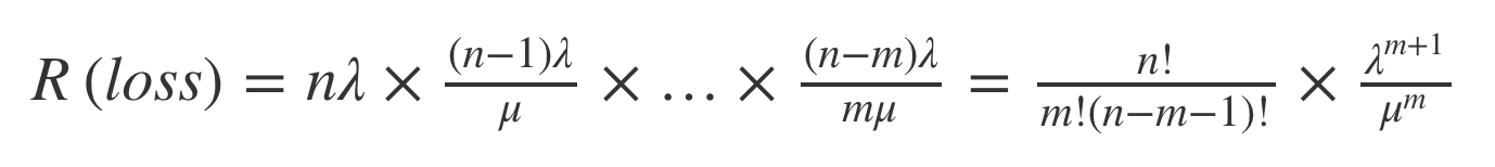
for a data loss rate of R(loss) replication groups per hour.
Let MTTF = 500000 hours for a SATA disk [3]. Let’s say MTTR = 24, which is the time to replace and re-replicate a disk after failure. If we adopt three-way data replication we have n = 3, m = 2, λ=1/500000, and μ=1/24.
Plugging these into the equation earlier, we get R(loss) = 1.3824 × 10^(–14) data loss incidents per hour or 5.04 × 10^(–12) incidents per year. This means that a given replication group is safe in a given year with probability 0.999999999994.
That is almost 11 nines right there.
Thing to note is that this is the rate for a single group. The error gets multiplied when you have multiple replication groups handling much more data. There is further math in paper [1,2,3,4] about efficient modelling of durability, and also how Tiered Replication provides more efficient results as it revolves around efficient replication using Copysets along with the concept of scatter time. I've linked the resources which had been really helpful.
References
[1] Copysets
[2] Tiered Replication
[3] Markov modelling of RAID systems
[4] Dropbox Magic Pocket
[5] Mean time to meaningless